we think about measurement

A little history

In 1831, the British physicist and chemist Michael Faraday enunciated a law of strategic importance for the future of electromagnetism and telecommunications. This law, called Faraday's Law of Induction or simply Faraday's Law, explained how a transient current could be induced in a conductor by a variable magnetic field, or, as we will see in more detail, by a conductor moving in a constant magnetic field.

The possibility of measuring a voltage induced by a moving fluid, subjected to a magnetic field, was already known to Faraday in 1832, he built a magnetic circuit to measure the flow of water that passed under the Waterloo Bridge in London, his design For the time it was unusual, it consisted of using the earth's own magnetic field and two metal sheets placed in the channel used as electrodes. The lack of instruments to measure with adequate sensitivity at the time, added to electrochemical effects, did not allow Farady to be successful, but the concept was successful. The first electromagnetic flow meter device was reported by Williams in 1930, Foxboro had the patent in 1952 and in 1954 the first instrument was released. In 1962 J. A. Schercliff published his work laying strong theoretical bases that describe his behavior.

Operating principle

Thanks to the studies postulated by Michael Faraday, these discoveries could not only be applied to telecommunications, but also to the measurement of fluids in motion.

To understand a little better the principle of operation of electromagnetic flowmeters, we will look at Faraday's law in more detail:

Faraday's Law of Induction:                                              ΔE=D.V.B

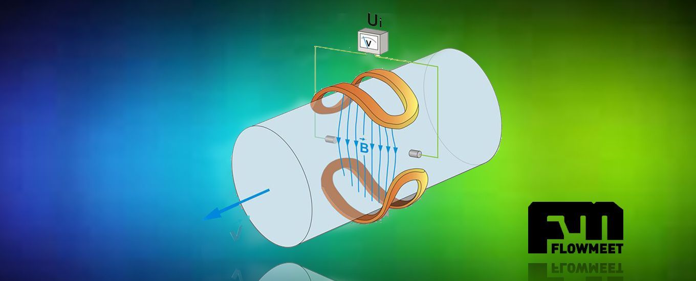
This law tells us that, if we move a conductor of diameter D within a magnetic field B at a speed V, we will obtain an induced emf (voltage) across this conductor. In other words, and getting closer to our interests, if we generate a magnetic field across the flow profile of a certain fluid, we will obtain a voltage. And more importantly, this voltage will be proportional to the speed of that fluid.Knowing this voltage and the diameter of the flow profile of the fluid (diameter of the pipe in which it travels) we can easily obtain its flow.

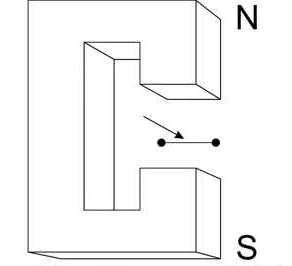
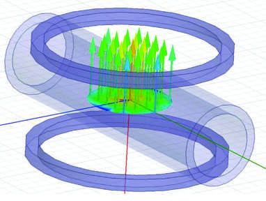
Two figures are shown below, the one on the left represents an experiment where the effect of Faraday's law could be measured, the one on the right shows a simulation of a pair of Helmholtz coils, the field should be as uniform as possible, this so that the response of the calimeter is linear, although the Helmholtz geometry presents a high linearity, it is not feasible for the construction of commercial flowmeters because the sensor would have a large size.

                                         

In an electromagnetic flowmeter two electrodes are placed tangentially in the pipe, the internal liquid links them if it is an electrical conductor, this galvanic union acts as the moving conductor. In the real case, it cannot be assumed that the signal from the electromagnetic flowmeter results from the application of Farday's law to the straight line joining both electrodes. We could think of as multiple fiber-forming paths of the liquid that joins both electrodes, something like what is shown in the following figure:

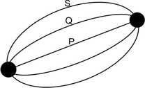
The paths S, Q and P do not only touch at the ends, they can be imagined as if they were the center of tubes that are in contact with each other with their surfaces in contact, the length of the paths are different, the speed of the fluid is different for different points in the profile of the pipe, to this it is added that the paths move away from the field of action of the coils, there will be different field strengths at the different points of each path, despite the fact that this description describes a complex emergent relationship between the flow rate and the potential difference, generated between the electrodes, with certain limitations it is possible to arrive at the aforementioned equation as the flow ratio and the electrical signal:

Resulting equation:  ΔE=D.V.B

ΔE Induced voltage between electrodes.
B Magnetic field.
D Pipe diameter.
V Average fluid velocity.

This equation is valid if the following is taken into account:

• The magnetic field is uniform in a certain region.

• The velocity of the fluid has a profile that is axial-symmetric.

The most critical point is the first, keeping the magnetic flux uniform is a challenge of considerable dimensions in current compact designs.

Flowmeter

Having seen a bit of history and a bit of theory of operation, now we are going to talk about the flowmeter.You would think that measuring the flow rate of a fluid shouldn't be complicated, but it is. Different pressures, temperatures, viscosities, conductivity, abrasiveness, composition, state of aggregation, etc. makes that for each problem there are only a limited number (or one ... or none) of solutions.Constructively, electromagnetic flowmeters can be divided into two parts, the sensor or primary element and the flow computer or secondary element, in what follows we will describe the primary sensor.

Because it has no moving or mechanical parts, it is maintenance-free equipment and the fact that it does not obstruct the flow makes it ideal for systems where disturbance is a limiting factor. It is totally immune to vibrations. It has an internal insulating coating (since the conductivity of the pipe would affect the measurement) that can be made of Neoprene, Teflon, PTFE, or other similar ones, which allows the fluid to be measured to be really hostile (very high / low pH, temperatures extremes -50 ° C to 200 ° C, mechanical abrasiveness) without affecting the durability of the equipment.

The versatility of the operating principle of this flowmeter allows it to be able to differentiate the direction of flow of the fluid, being one of the few measurement technologies that is not only indifferent when measuring flow, but it can differentiate them in the case that is of interest to the user.

One aspect to highlight in this type of flow meter is the measurement interval since, for a given model, the maximum flow becomes 100 times higher than the minimum.The measurement error of this type of flow meter is around 0.5% and at the customer's request it can be 0.2%.

Conclusions

Due to all the aforementioned advantages, the electromagnetic flowmeter is the third most widely used flowmeter in the industry.